作者:陈广 日期:2019-10-7
最终还是决定自已写一个 QR 码绘制程序,难点在于纠错码的计算,虽然可以在网上找算法包,但还是需要了解这方面的知识。在网上找到一篇相当不错的文章,英文的,老外写的就是通俗易懂!于是决定将其翻译。这一块是不可能写在书上的,已经超出高职学生的接受能力。放在网上,给有能力学的同学参考吧。文章是用 Python 写的代码,我的想法是将其翻译成 C# 代码,这个没什么难度。之前培训时学过半天的 Python,说实在的,我不太喜欢这类动态语言,不过用它来做一些数学计算还是挺方便的。虽然要写 Python 代码可能要费些周折,但只是读代码,成本几乎就为 0 了。运行 Python 只需在网上下载 Python 环境并安装。然后 Visual Studio Code 加入相应的插件就可以用了,非常方便。
原文链接:https://en.wikiversity.org/wiki/Reed–Solomon_codes_for_coders
纠错码是一种用于纠错的信号处理技术。它们无处不在,例如通信(手机、互联网)、数据存储和存档(硬盘驱动器、光盘CD/DVD/蓝光、档案磁带)、仓库管理(条码)和广告(QR 码)。
Reed–Solomon 纠错码是一种特殊类型的纠错码。它是最古老的一种纠错类型,但现今仍被广泛使用,它是应用于公共领域的优秀的几种高效算法之一。
通常,纠错码隐藏在幕后,大多数用户甚至不了解它们,也不知道它们在何时使用。然而,它们是某些应用程序得以运行的关键部件,例如通信或数据存储。事实上,每隔几天随机便会丢失数据的硬盘将是无用的,只有在晴朗天气才能打电话的手机将很少被使用。使用纠错码可以将损坏的消息恢复为完整的原始消息。
条码和 QR 码是值得研究的有趣应用,因为它们具有直观显示纠错码的功能,好奇的用户可以轻而易举地翻译这些代码以供访问。
本文试图从程序员而非数学家的角度介绍 Reed–Solomon 码的原理,这意味着我们将更多地关注实践而不是理论,虽然我们也将解释理论,但仅针对那些对感知和实现有必要的知识。我将提供领域中的重要参考资料,以便感兴趣的读者可以深入了解数学理论。我们将通过流行的 QR 码系统提供现实世界的例子,以及代码样本。我们选择使用 Python 作为示例(主要是因为它看起来很漂亮,并且类似于伪代码),但是我们将尝试为那些不熟悉 Python 的人解释任何不明显的特性。其中所涉及的数学是高级的,它通常在大学才会教授,但一个较好掌握高中代数的人应该可以理解。
首先,我们将轻松地介绍纠错码原理背后的感性知识,然后在第二节中,我们将介绍 QR 码的结构设计,换句话说,信息是如何存储在 QR 码中的,以及如何读取和生成它;在第三节中,我们将通过实现 Reed–Solomon 解码器来研究纠错码,并快速介绍更宏大的 BCH 码系列,以便可靠地读取损坏的 QR 码。
请注意,对于好奇的读者来说,扩展的信息可以在附录和讨论页中找到。
在详细说明代码之前,了解纠错背后的感性知识是非常有用的。事实上,尽管纠错码在数学上似乎令人望而生畏,但大多数数学运算都是高中级别的(除 Galois Fields 外,实际上对任何程序员来说都很简单和常见:它只是简单地将整数与一个数字进行模操作)。然而,纠错码背后的数学智慧的复杂性掩盖了相当直观的目标和作用机制。
纠错代码似乎是一个困难的数学概念,但它们实际上是基于一个直观的想法,并有一个巧妙的数学实现:将数据结构化,当数据损坏时,通过“修复”结构,我们可以“猜测”数据是什么。 从数学上讲,我们使用 Galois Fields(伽罗华域)中的多项式来实现这个结构。
让我们来做一个更实际的类比:假设您想要将消息传递给其他人,但是这些消息可能会在此过程中损坏。纠错码的主要想法是:使用较小的由一组精心挑选的单词组成的“简化字典”,而不是使用整本字典,以使每个单词有别于其它单词。 这样,当收到消息时,只需在简化字典中查找:
我们来举一个简单的例子:有一本简化字典,只有三个由 4 个字母组成的单词:this、that和corn。假设我们收到了一个损坏的单词:co**,*表示丢失的字母。由于字典中只有 3 个单词,我们可以很容易地将收到的单词与的字典进行比较,以找到最接近的单词。本例中,它是corn。因此,丢失的字母是rn。
现在,假设收到的单词是th**,问题是字典中有两个匹配的单词:this和that。这种情况下,无法确定是哪个单词,导致解码失败。这意味着字典不够好,我们应当使用更为不同的单词替换that,如dash,以最大限度地扩大每个单词之间的差异。这种差异,或者更准确地说,是字典中任意两个单词之间不同字母的最小数量,称为字典的最大汉明距离。确保字典中的任意两个单词在同一位置上只共享最少数量的字母称为最大可分性。
大多数纠错码都使用相同的原理:我们只生成一个简单字典,其中只包含具有最大可分性的单词(我们将在第三节中详细说明如何做到这一点),然后我们只使用该简化字典中的单词进行通信。伽罗华域提供的是结构(即,简化字典基础),Reed–Solomon 是一种自动创建适当结构的方法(为数据集定制最大可分性的简化字典),以及提供自动方法来检测和纠错(即,在简化字典中查找)。更准确地说,伽罗华域是一种结构(由于它们的循环性质,与整数进行模运算),Reed–Solomon 是基于伽罗华域的编/解码器。
如果一个单词在通信中损坏则问题不大,因为我们可以通过查找字典并找到最接近的单词来轻松地解决它,这可能是正确的(但是,如果输入消息损坏太严重,就有可能选择一个错误的词,但概率很小)。而且,我们的单词越长,它们的可分性就越高,因为有更多的字符可以被破坏而不产生任何影响。
生成最大可分字典的最简单方法是使单词比实际更长。
我们再次举例:
t h i s
t h a t
c o r n
追加一组独特的字符,以便在任意追加位置都不存在重复字符,并添加一个单词以帮助解释:
t h i s a b c d
t h a t b c d e
c o r n c d e f
请注意,字典中的每个单词与其他单词至少有 5 个字符不同,因此距离为 5。这使得在已知位置上最多有 4 个错误(称为擦除错误),或两个未知位置的错误需要纠正。
译者注:我数来数去,应当有 6 个单词不同才对啊?。
假设有 4 个擦除错误:
t * * * a b * d
然后查找字典以对 4 个未被擦除的字符进行搜索,找到与这 4 个字符匹配的唯一条目,由于距离为 5,结果为:t h i s a b c d。
假设在某一模式中发生两个错误:
t h o s b c d e
这里的问题是错误的位置是未知的。我们再次进行字典搜索:8 个字符中包含 6 个字符的子集数为 28,因此将一一使用 28 个 6 字符子集进行搜索,而且由于距离为 5(假设出现了 2 个或更少的错误),只会有一个匹配 6 个字符的子集。本例为:t h a t b c d e。
通过这些示例,可以看到冗余在恢复丢失信息方面的优势:冗余字符可以帮助您恢复原始数据。前面的例子粗略地显示了纠错方案是如何工作的。Reed–Solomon 的核心思想类似,基于数学上的伽罗华域向一条信息附加冗余数据。原始纠错解码器类似于上面的错误示例,搜索与有效消息相对应的接收消息的子集,并选择最匹配的一个作为校正消息。对于较长的消息来说,这是不实际的,因此开发了数学算法,以便在合理的时间内执行错误校正。
本节介绍 QR 码结构,也就是数据是如何存储在 QR 码中的。本节中的信息并不完整。这里只介绍了 21×21 尺寸符号(也称为版本1)最常见的特性,但请参阅附录以获得更多信息。
以下是一个将要作为示例的 QR 符号。它由黑色及浅色方块组成(在条码世界被称为模块),角上的三个矩形位置探测图形是 QR 符号的视觉特征。

掩模过程用于避免符号中可能会混淆扫描仪的特征,例如看起来像位置探测图形的误导形状和较大的空白区域。掩模反转某些模块(白色变成黑色,黑色变成白色),而不让其他模块单独使用。
在下图中,红色区域表示格式信息并使用固定的掩模图案。数据区域(黑白)以可变图案掩模。当代码被创建时,编码器尝试多个不同的掩码,并选择了结果中不良特征最小化的掩码。然后,在格式信息中指示所选择的掩码图案,以便解码器知道要使用哪一个。浅灰色区域是固定的案,不编码任何信息。除了明显的位置探测图形,还有包括模块深浅交替的定位图形。
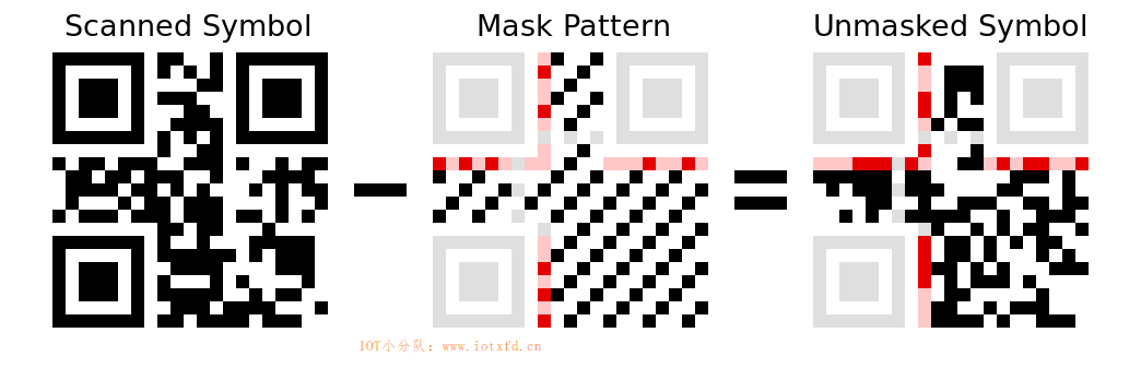
掩模转换很容易应用或移除,因为它使用的是异或操作(大多数编程语言中使用插入符号^表示)。未掩模的格式信息如下所示。按逆时针方向读取左上方的位置探测图形周围,我们得到以下的位序列:白色模块代表 0,黑色模块代表 1。
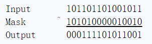
译者注:第一行 Input 数值实际是读取上图 Scanned Symbol 图案中的格式信息部分,注意中间有两个黑块属定位图形,请跳过不读;第二行 Mask 数值读取的是上图 Mask Pattern 图案中的格式信息部分;第三行数值是经过前两行异或运算得出,也可读取上图 Unmasked Symbol 图案中的格式信息部分。
格式信息有两个相同的副本,因此即使符号已损坏,也可以对其进行解码。第二份拷贝被分成两部分,放在另外两个位置探测图形周围,并按逆时针方向读取(左下角向上,右上角从左到右)。
格式信息的前两位给出用于消息数据的纠错级别。这个版本的 QR 符号包含 26 个字节的信息。其中一部分用于存储消息,另一部分用于纠错,如下表所示。左边列是纠错级别名称。
| 纠错等级 | 等级指示符 | 纠错码字节数 | 数据码字节数 |
|---|---|---|---|
| L | 01 | 7 | 19 |
| M | 00 | 10 | 16 |
| Q | 11 | 13 | 13 |
| H | 10 | 17 | 9 |
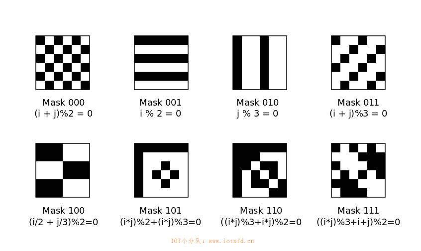
格式信息中的下三位选择要在数据区域中使用的掩模图案。这些图案如下所示,包括一个模块是否是黑色的数学公式(i 和 j 分别是行数和列数,从左上角的 0 开始)。
格式信息中的其余 10 位用于纠正格式本身的错误。这一点将在后面的一节中解释。
这是一个更大的图像,显示了“未掩模” 的 QR 码。指示符号的不同区域,包括信息数据字节的边界。
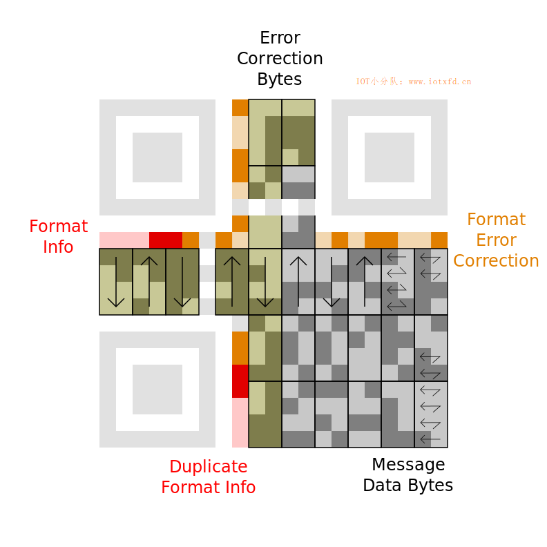
从右下角开始读取数据位,并以锯齿形模式延两个右侧列向上移动。前三个字节为:01000000 11010010 01110101。接下来的两列向下读取,所以接下来的字节是01000111。到达底部后,下两列向上读取。以这种上下交错的方式进行,一直到符号的左边(必要时跳过定位图形)。以下是十六进制表示的完整消息:
信息数据字节:40 d2 75 47 76 17 32 06 27 26 96 c6 c6 96 70 ec
纠错字节:bc 2a 90 13 6b af ef fd 4b e0
最后一步是将信息字节解码为可读的内容。前四位指示如何对消息进行编码。QR 码采用多种不同的编码方案,以便高效地存储不同类型的消息。下表概述了这些情况。模式指示符之后是一个长度字段,它显示存储了多少个字符。长度字段的大小取决于特定的编码。
| 模式名称 | 模式指示符 | 长度位数 | 数据位数 |
|---|---|---|---|
| 数字 | 0001 | 10 | 每3个数字10位 |
| 字母数字 | 0010 | 9 | 每2个字符11位 |
| 字节 | 0100 | 8 | 每字符8位 |
| 日本汉字 | 1000 | 8 | 每字符13位 |
(以上长度字段大小仅对版本较小的 QR 码有效。)
我们的示例信息以0100开头,表示每个字符占用 8 个位。接下来的 8 位是长度字段:00001101或十进制的 13。之后是信息的实际字符。前两个是00100111和01010100(单引号和T的 ASCII 码)。有兴趣的读者可以自己解码其余的信息。
最后一个数据位之后是另一个 4 位模式指示符。它可以与第一个不同,允许在同一个 QR 符号中混合不同的编码。当没有更多的数据可存储时,就会给出特殊的终止符0000。(请注意,如果数据字节可用数量不足,允许省略终止符。)
此刻,我们已经知道如何解码或读取整个 QR 代码。然而,在现实生活中,QR 代码很少是完整的:通常,它是通过手机摄像头在恶劣的照明条件下,或者在部分 QR 代码被扯破的表面上,或者在有污点表面上进行扫描的。
为了使我们的 QR 码解码器可靠,我们需要能够纠正错误。本文的下一部分将描述如何通过构造 BCH 解码器,特别是 Reed–Solomon 解码器来纠正错误。
本节,我们介绍一类常见的纠错码:BCH 码,现代 Reed–Solomon 码的祖先,以及基本的检测和校正机制。
格式化信息使用 BCH 进行编码,允许检测和纠正一定数量的位错误。BCH 码是 Reed–Solomon 码的普通版(现代 Reed–Solomon 码是 BCH 码)。在 QR 码中,用于格式信息的 BCH 码比用于信息数据的 Reed–Solomon 码简单得多,因此从格式信息的 BCH 代码开始是有意义的。
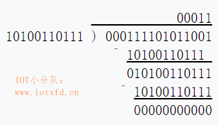
检查编码信息的过程类似于长除法,但使用异或代替减法。当格式码被所谓的编码生成器“除”时,它应该产生一个零的余数。QR 格式码使用生成码10100110111。以下示例的格式信息码(0001111011001)演示了这个过程。
下面是实现此计算的 Python 函数:
def qr_check_format(fmt):
   g = 0x537 # = 0b10100110111 in python 2.6+
   for i in range(4,-1,-1):
      if fmt & (1 << (i+10)):
         fmt ^= g << i
   return fmt
Python 注解:
range函数对于非 Python 程序员可能比较陌生。它产生一个 4 到 0 的数字列表。在类 C 语言中,for循环语句应写为:for(i=4;i>=0;i--);在类 Pascal 语言中为:for i := 4 downto 0。
Python 注解2:
&操作符执行按位与,<<为左移。这与类 C 语言是一致的。
此函数还可用于对5位格式信息进行编码。
encoded_format = (format<<10) ^ qr_check_format(format<<10)
读者可能会发现一个有趣的练习,把这个函数推广到除以不同的数字。例如,版本号高的 QR 码包含 6 位版本信息以及 12 位纠错码,所使用的生成码为:1111100100101。
在数学形式中,这些二进制数被描述为多项式,其系数是整数模2。该数的每一位都是一个项的系数。例如:
$10100110111 =$ $ 1 x^{10} + 0 x^9 + 1 x^8 + 0 x^7 + 0 x^6$ $+ 1 x^5 + 1 x^4 + 0 x^3 + 1 x^2 + 1 x + 1$ $= x^{10} + x^8 + x^5 + x^4 + x^2 + x + 1$
如果qr_check_format生成的余数不是零,则代码已被损坏或误读。下一步是确定哪种格式代码最有可能是预期的格式码(即在我们的简化字典中查找)。
虽然有复杂的 BCH 解码算法存在,但在这种情况下使用它们是杀鸡用牛刀。由于只有 32 种可能的格式码,所以简单地尝试每种编码并选择与所述编码不同位数最小的编码(不同位数量称为汉明距离)要容易得多。这种查找最接近的编码的方法被称为穷尽搜索,并且只是编码数量非常少才有可能(编码为有效的消息的个数只有 32,所有其他二进制数字都是不正确的)。
注意:Reed–Solomon 也是基于这一原则,但由于可能的码字数量太大,负担不起进行详尽的搜索,这就是为什么聪明但复杂的算法被设计出来,如 Berlekamp-Massey。
def hamming_weight(x): #计算一个二进制数中 1 的个数
   weight = 0
   while x > 0:
      weight += x & 1
      x >>= 1
   return weight

def qr_decode_format(fmt):
   best_fmt = -1
   best_dist = 15
   for test_fmt in range(0,32):
      test_code = (test_fmt<<10) ^ qr_check_format(test_fmt<<10)
      test_dist = hamming_weight(fmt ^ test_code)
      if test_dist < best_dist:
         best_dist = test_dist
         best_fmt = test_fmt
      elif test_dist == best_dist:
         best_fmt = -1
   return best_fmt
如果格式码不能被明确解码,函数qr_decode_format将返回 -1。当两个或多个格式码与输入的距离相同时,就会发生这种情况。
要在 Python 中运行这些代码,首先启动 Python 的集成开发环境(本人使用的是 Visual Studio Code)。新建一个名为 qr.py 的文件,拷贝qr_check_format,hamming_weight以及qr_decode_format函数进去并保存。返回命令提示符并输入python命令,您将看到版本信息以及交互式输入提示符>>>。输入如下命令:
>>> from qr import *
>>> qr_decode_format(int("000111101011001",2))  # no errors
3
>>> qr_decode_format(int("111111101011001",2))  # 3 bit-errors
3
>>> qr_decode_format(int("111011101011001",2))  # 4 bit-errors
-1
在接下来的章节中,我们将研究有限域算法和 Reed–Solomon 码,这是 BCH 码的一个子类型。基本思想是一样的(即使用具有最大可分性的有限单词字典),但是由于我们将编码更长的单词(256个字节而不是2个字节),有更多的符号可用(编码在所有8位上,因此有256个不同的可能值),不能使用这种天真的、详尽的方法,因为它需要花费太多的时间:我们需要使用更聪明的算法,有限域数学将通过一个结构来帮助我们做到这一点。
在讨论用于信息的 Reed–Solomon 码之前,介绍一些更多的数学知识将是有用的。
我们定义 8 位字节的加、减、乘、除,结果总是产生 8 位字节,以避免任何溢出。我们可能天真地尝试使用这些操作的正常定义,然后与 256 进行取模运算,以防止结果溢出。这正是我们将要做的,也就是所谓的伽罗华域 2^8。你可以很容易地想象它为什么适用于所有事物,除了除法:7/5是多少?
以下是对伽罗华域的简要介绍:有限域是一组数字,域需要有六个属性:封闭、结合、交换、分布、恒等和逆。更简单地说,使用域允许研究该域的数字之间的关系,并将结果应用于遵循相同属性的任何其他域。例如,实数集 ℝ 是一个域。换句话说,数域研究一组数字的结构。
然而,整数 ℤ 不是一个域,因为正如我们前面所说,并非所有的除数都是定义的(例如7/5),这违反了乘法逆属性(例如,对于整数 x 来说,7*x=5 不存在)。解决这个问题的一个简单方法是使用素数进行取模运算,如 2:这样,我们就可以保证7*x=5的存在,因为我们只需要绕一圈就行了。ℤ % 2 叫伽罗华域,任何可被 2 除的数都是伽罗华域(因为我们需要使用素数进行取模运算),因此,256,一个8位符号的值,可以减少到$2^8$,因此我们说我们使用 $2^8$ 的伽罗华域,或 $GF(2^8)$。在口语中,2是域的特征,8是指数,256是域的基数。有关有限域的更多信息可以在这里找到。
接下来我们将定义通常的数学操作,通常使用整数,但适合于 $GF(2^8)$,它基本上是做通常的操作,但与 $2^8$ 进行取模运算。
另一种思考 $GF(2)$ 和 $GF(2^8)$ 之间联系的方法是认为 $GF(2^8)$ 表示一个 8 位二进制系数的多项式。例如,在 $GF(2^8)$ 中,170 等价于
$10101010 =$ $1 \times x^7 + 0 \times x^6 + 1 \times x^5$ $+ 0 \times x^4 + 1 \times x^3 + 0 \times x^2 + 1 \times x + 0$ $= x^7 + x^5 + x^3 + x$
这两种表示都是等价的,只是在第一种情况下,170 表示的是十进制,而在另一种情况下,它是二进制的,可以被认为是按照惯例表示多项式(仅用于 $GF(2^p)$,如这里所解释的)。后者通常是学术书籍和硬件实现中使用的表示形式(因为逻辑门和寄存器在二进制级别工作)。对于软件实现,十进制表示是首选,它更清晰、更接近于数学代码。这是我们将在本教程中使用的代码,除了一些将使用二进制表示的示例之外。
无论如何,不要混淆表示单个 $GF(2^p)$ 符号的多项式(每个系数是位/布尔值:0或1),以及表示 $GF(2^p)$ 符号列表的多项式(在这种情况下,多项式等价于 信息+RScode,每个系数是 0 到 $2^p$ 之间的值,并表示 信息+RScode 的一个字符)。我们首先描述单个符号上的操作,然后对一个符号列表进行多项式运算。
在以 2 为基的伽罗华域中,加法和减法都被异或运算取代。逻辑为:加法模 2 等价于 XOR,减法模 2 等价于加法模 2。这是可能的,因为加减法在此伽罗华域中不进位。
把我们的 8 位值看作系数 mod 2 的多项式:
0101 + 0110 = 0101 - 0110 = 0101 XOR 0110 = 0011
同样的方式为(在两个单个 $GF(2^8)$ 整数的二进制表示中):
$(x^2 + 1) + (x^2 + x) $ $= 2 x^2 + x + 1$ $= 0 x^2 + x + 1 = x + 1$
因为(a ^ a) = 0(这里的 ^ 是异或操作),每个数字都是它自己的对立面,所以x - y与x + y相同。
请注意,在书中,您将找到加法和减法来定义 GF 整数上的一些数学运算,但在实践中,您可以只进行 XOR(只在基为 2 的伽罗华域中有效,在其他域中就不是这样了)。
下面是等效的 Python 代码:
def gf_add(x, y):
    return x ^ y

def gf_sub(x, y):
    return x ^ y # in binary galois field, subtraction is just the same as addition (since we mod 2)
乘法同样是基于多项式乘法的。简单地将输入写成多项式,然后用基于分配律将它们相乘。例如,计算10001001乘以00101010如下。
$(x^7 + x^3 + 1) (x^5 + x^3 + x)$ $= x^7 (x^5 + x^3 + x) + x^3 (x^5 + x^3 + x) + 1 (x^5 + x^3 + x)$ $= x^{12} + x^{10} + 2 x^8 + x^6 + x^5 + x^4 + x^3 + x$ $= x^{12} + x^{10} + x^6 + x^5 + x^4 + x^3 + x$
同样的结果可以通过修正的标准小学乘法程序得到,在这个过程中,我们用异或替代加法。
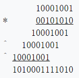
注意:这里的 XOR 乘法是不进位的!如果你使用进位,会得到错误的结果:携带$x^9$项的
1011001111010,而不是正确的结果1010001111010。
以下是一个 Python 函数,它在单个$GF(2^8)$整数上实现了这个多项式乘法。
注意:这个函数(和下面的一些其他函数)使用了很多位操作符,例如
>>和<<,因为它们可以更快、更简洁地完成我们想做的事情。这些运算符在大多数语言中都是可用的,它们并不是 Python 特有的,您可以在这里获得更多关于它们的信息。
def cl_mul(x,y):
    '''Bitwise carry-less multiplication on integers'''
    z = 0
    i = 0
    while (y>>i) > 0:
        if y & (1<<i):
            z ^= x<<i
        i += 1
    return z
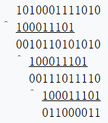
当然,结果不再适合8位字节(在本例中,它的长度为13位),因此我们需要在完成之前再执行一步。将结果与100011101取模进行简化(这个数字的选择在代码下面解释),使用前面描述的长除法过程。此种情况被称为“模降”,因为我们所做的基本上是使用模运算来划分和保留余数。在示例中,这将产生最后的答案11000011。
下面是 Python 代码来完成整个伽罗华域的乘法,并进行模降:
def gf_mult_noLUT(x, y, prim=0):
    '''在伽罗华域中进行乘法,且不使用预先计算的查找表(因此它更慢)
       利用不可约素多项式的标准无进位乘法 + 模降'''

    ### 将位无进位位操作定义为内部函数 ###
    def cl_mult(x,y):
        '''整数上的位无进位乘法'''
        z = 0
        i = 0
        while (y>>i) > 0:
            if y & (1<<i):
                z ^= x<<i
            i += 1
        return z

    def bit_length(n):
        '''计算整数的最靠左的 1 的位置。等效于 int.bit_length()'''
        bits = 0
        while n >> bits: bits += 1
        return bits

    def cl_div(dividend, divisor=None):
        '''按位对整数进行无进位长除法,并返回余数。'''
        # 计算每个整数的最靠左的 1 的位置
        dl1 = bit_length(dividend)
        dl2 = bit_length(divisor)
        # 如果被除数小于除数,就退出
        if dl1 < dl2:
            return dividend
        # 否则,将除数最左边的 1 与被除数最左边的 1 对齐(通过左移除数)。
        for i in range(dl1-dl2,-1,-1):
            # 检查被除数是否可除尽(对第一次迭代无效,但对下一次迭代很重要)。
            if dividend & (1 << i+dl2-1):
                # 如果可除尽,则将除数左移到对齐最左边 1 位并 XOR(无进位减法)。
                dividend ^= divisor << i
        return dividend

    ### 主 GF 乘法例程 ###

    # GF 数相乘
    result = cl_mult(x,y)
    # 然后用不可约素多项式进行模降(即除法中的余数),使其保持在gf界内。
    if prim > 0:
        result = cl_div(result, prim)

    return result
结果:
>>> a = 0b10001001
>>> b = 0b00101010
>>> print(bin(gf_mult_noLUT(a, b, 0))) # multiplication only
0b1010001111010
>>> print(bin(gf_mult_noLUT(a, b, 0x11d))) # multiplication + modular reduction
0b11000011
为何要使用100011101(16进制的 0x11D)取模?这里的数学有点复杂,但简单地说,100011101表示的是一个 8 次多项式,它是“不可约的”(意思是它不能表示为两个较小多项式的乘积)。这个数字被称为本原多项式或不可约多项式或素多项式(我们将在本教程的其余部分主要使用后一个名称)。这是必要的除法的良好行为,它帮助生成保持在伽罗华域的范围内,但不重复的值。还有其他我们可以选择的数字,但它们本质上都是一样的,100011101(0x11d)是 Reed–Solomon 码的一个常见的本原多项式。如果您想知道如何生成这些素数,请参阅附录。
关于素多项式的附加信息(你可以跳过):什么是素多项式?它在伽罗华域相当于一个素数。请记住,伽罗华域使用的值是 2 的倍数作为生成器。当然,在标准算术中,素数不能是 2 的倍数,但在伽罗华域是可能的。为什么我们需要素多项式?这是为了保持域的界限,我们需要计算伽罗华域之上任何值的模。为什么我们不直接和伽罗华域的阶取模呢?因为我们最终会得到很多重复的值,我们希望在域中有尽可能多的唯一值,这样一个数字在使用素多项式取模或 XOR 时总是有一个以及唯一的投影。
对感兴趣的读者请注意:作为一个例子,您可以使用巧妙的算法实现 GF 数的乘法,这里有另一种方法可以更简洁、更快地实现 GF 数的乘法,即 Russian Peasant Multiplication algorithm:
def gf_mult_noLUT(x, y, prim=0, field_charac_full=256, carryless=True):
    '''Galois Field integer multiplication using Russian Peasant Multiplication algorithm (faster than the standard multiplication + modular reduction).
    If prim is 0 and carryless=False, then the function produces the result for a standard integers multiplication (no carry-less arithmetics nor modular reduction).'''
    r = 0
    while y: # while y is above 0
        if y & 1: r = r ^ x if carryless else r + x # y is odd, then add the corresponding x to r (the sum of all x's corresponding to odd y's will give the final product). Note that since we're in GF(2), the addition is in fact an XOR (very important because in GF(2) the multiplication and additions are carry-less, thus it changes the result!).
        y = y >> 1 # equivalent to y // 2
        x = x << 1 # equivalent to x*2
        if prim > 0 and x & field_charac_full: x = x ^ prim # GF modulo: if x >= 256 then apply modular reduction using the primitive polynomial (we just subtract, but since the primitive number can be above 256 then we directly XOR).

    return r
请注意,使用参数prim=0和carryless=false的最后一个函数将返回标准整数乘法的结果(因此您可以看到无进位加法和带进位加法之间的区别及其对乘法的影响)。
上面描述的过程并不是实现伽罗华域乘法的最方便的方法。乘两个数需要乘法循环的 8 次迭代,然后是最多 8 次的除法循环。但是,通过使用查找表,我们可以在没有循环的情况下进行乘法。一种解决方案是在内存中构造整个乘法表,但这需要一个庞大的 64k 表。下面描述的解决方案要紧凑得多。
首先,请注意,乘 2=00000010(按照惯例,这个数字称为α或生成器号)只需使用左移一位来替代,然后在必要时使用模数100011101进行异或运算(此种情况下,xor 为何满足取模运算则留给读者自行思考)。以下是α的最初的几个幂。
| $\alpha^0 = 00000001$ | $\alpha^4 = 00010000$ | $\alpha^8 = 00011101$ | $\alpha^{12} = 11001101$ |
| $\alpha^1 = 00000010$ | $\alpha^5 = 00100000$ | $\alpha^9 = 00111010$ | $\alpha^{13} = 10000111$ |
| $\alpha^2 = 00000100$ | $\alpha^6 = 01000000$ | $\alpha^{10} = 01110100$ | $\alpha^{14} = 00010011$ |
| $\alpha^3 = 00001000$ | $\alpha^7 = 10000000$ | $\alpha^{11} = 11101000$ | $\alpha^{15} = 00100110$ |
如果以相同的方式继续使用此表,则α的幂在$\alpha ^{255}=00000001$之前不会重复。因此,除零外,场中的每一个元素都等于α的某种幂。我们定义的元素α被称为伽罗华域的本原元或生成器。
这一观察提出了另一种实现乘法的方法:通过添加α的指数。
$10001001 \times 00101010$ $= \alpha^{74} \times \alpha^{142}$ $= \alpha^{74 \times 142} = \alpha^{216} = 11000011$
问题是,我们如何找到与10001001相对应的α的幂?这就是所谓的离散对数问题,而且不知道有效的通解。然而,由于这个域中只有256个元素,所以我们可以很容易地构造一个对数表。当我们完成它时,相应的逆对数表(指数)也将是有用的。关于这个技巧的更多数学信息可以在这里找到。
gf_exp = [0] * 512 # 创建512个元素的列表,考虑使用字节数组
gf_log = [0] * 256

def init_tables(prim=0x11d):
    '''预先计算对数表和逆对数表,以便以后使用所提供的本原多项式进行更快的计算。'''
    # 素数是本原(二元)多项式。因为它是二元意义上的多项式,
    # 实际上,它只是0到255之间的一个伽罗华域值,而不是 GF 值的列表。
    global gf_exp, gf_log
    gf_exp = [0] * 512 # 逆对数(指数)表
    gf_log = [0] * 256 # 日志表
    # 对于伽罗华域 2^8 中的每个可能值,我们将预先计算该值的对数和反对数(指数)。
    x = 1
    for i in range(0, 255):
        gf_exp[i] = x # 计算此值的逆对数并将其存储在表中。
        gf_log[x] = i # 同时计算对数
        x = gf_mult_noLUT(x, 2, prim)

        # 如果只使用生成器=2或幂为2,则可以使用以下比gf_mult_nolut()更快的方法:
        #x <<= 1 # multiply by 2 (change 1 by another number y to multiply by a power of 2^y)
        #if x & 0x100: # similar to x >= 256, but a lot faster (because 0x100 == 256)
            #x ^= prim # substract the primary polynomial to the current value (instead of 255, so that we get a unique set made of coprime numbers), this is the core of the tables generation

    # 优化:使逆对数表的大小加倍,这样我们就不需要使用 mod 255
    # 保持在边界内(因为我们将主要使用这个表来计算两个 GF 数的乘法)
    for i in range(255, 512):
        gf_exp[i] = gf_exp[i - 255]
    return [gf_log, gf_exp]
Python 注解:
ragne运算符的上界是排他性的,因此gf_exp[255]不会被上面设置两次。
为了简化乘法函数,gf_exp表的尺寸放大。这样,我们就不必检查gf_log[x] + gf_log[y]是否在表界限之内。
def gf_mul(x,y):
    if x==0 or y==0:
        return 0
    return gf_exp[gf_log[x] + gf_log[y]] # should be gf_exp[(gf_log[x]+gf_log[y])%255] if gf_exp wasn't oversized
对数表法的另一个优点是它允许我们用对数的差异来定义除法。在下面的代码中,添加255以确保差不是负的。
def gf_div(x,y):
    if y==0:
        raise ZeroDivisionError()
    if x==0:
        return 0
    return gf_exp[(gf_log[x] + 255 - gf_log[y]) % 255]
Python 注解:
raise语句抛出一个异常,并中止gf_div函数的执行。此除法,gf_div(gf_mul(x,y),y)==x,对于任何 x 和任何非零 y 有效。
更高级的程序员读者可能会发现编写一个封装伽罗华域算法的类很有趣。操作符重载可以用熟悉的操作符*和/替换对gf_mul和gf_div的调用,但这会导致对正在执行的操作类型的混淆。某些细节可以使类以更广泛有用的方式加以概括。例如,Aztec 代码使用 5 个不同的伽罗华域,元素大小从 4 位到 12 位不等。
在计算幂和逆时,对数表法将再次简化和加速我们的计算:
def gf_pow(x, power):
    return gf_exp[(gf_log[x] * power) % 255]

def gf_inverse(x):
    return gf_exp[255 - gf_log[x]] # gf_inverse(x) == gf_div(1, x)
在讨论 Reed–Solomon 码之前,我们需要对系数为伽罗华域元素的多项式定义几个运算。这是一个潜在的混乱根源,因为元素本身被描述为多项式;我的建议是不要想得太多。更令人困惑的是,x仍然用作占位符。这个x与前面提到的x无关,所以不要混淆它们。
以前用于伽罗华域元素的二进制表示法在此时开始变得笨重起来,因此我将改用十六进制。
$00000001 x^4 + 00001111 x^3 + 00110110 x^2$ $+ 01111000 x + 01000000$ $= 01 x^4 + 0f x^3 + 36 x^2 + 78 x + 40$
在 Python 中,多项式将由幂降序x数列表示,因此上面的多项式成为[ 0x01, 0x0f, 0x36, 0x78, 0x40 ]。可以使用相反的顺序;这两种选择各有优缺点。
第一个函数将多项式乘以标量。
def gf_poly_scale(p,x):
    r = [0] * len(p)
    for i in range(0, len(p)):
        r[i] = gf_mul(p[i], x)
    return r
Python 程序员注意:此函数不是以“pythonic”样式编写的。它可以很优雅地表达为一个列表推导式,但我限制自己的语言特性,更容易翻译到其他编程语言。
此函数“添加”两个多项式(使用异或,如往常一样)。
def gf_poly_add(p,q):
    r = [0] * max(len(p),len(q))
    for i in range(0,len(p)):
        r[i+len(r)-len(p)] = p[i]
    for i in range(0,len(q)):
        r[i+len(r)-len(q)] ^= q[i]
    return r
下一个函数将两个多项式相乘。
def gf_poly_mul(p,q):
    '''Multiply two polynomials, inside Galois Field'''
    # Pre-allocate the result array
    r = [0] * (len(p)+len(q)-1)
    # Compute the polynomial multiplication (just like the outer product of two vectors,
    # we multiply each coefficients of p with all coefficients of q)
    for j in range(0, len(q)):
        for i in range(0, len(p)):
            r[i+j] ^= gf_mul(p[i], q[j]) # equivalent to: r[i + j] = gf_add(r[i+j], gf_mul(p[i], q[j]))
                                                         # -- you can see it's your usual polynomial multiplication
    return r
最后,我们需要一个函数在x的特定值下求一个多项式,从而产生一个标量结果。利用 Horner 方法避免显式计算x的幂。Horner 方法通过连续分解这些项来工作,因此我们总是迭代地处理x^1,从而避免了高次项的计算:
$01 x^4 + 0f x^3 + 36 x^2 + 78 x + 40$ $= (((01 x + 0f) x + 36) x + 78) x + 40$
def gf_poly_eval(poly, x):
    '''Evaluates a polynomial in GF(2^p) given the value for x. This is based on Horner's scheme for maximum efficiency.'''
    y = poly[0]
    for i in range(1, len(poly)):
        y = gf_mul(y, x) ^ poly[i]
    return y
我们还需要一个缺失的多项式运算:多项式除法。这比多项式上的其他运算要复杂得多,所以我们将在下一章和 Reed–Solomon 编码一起研究它。
现在,准备就绪,我们准备开始研究 Reed–Solomon 码。
但首先,为什么我们要学习有限域和多项式?因为这是像 Reed–Solomon 这样的纠错代码的主要洞察力:我们不只是把一条信息看作一系列(ASCII)数字,而是把它看作一个多项式,遵循有限域算法中定义得很好的规则。换句话说,通过用多项式和有限域算法来表示数据,我们在数据中增加了一个结构。消息的值仍然相同,但是这个概念结构现在允许我们使用定义良好的数学规则对信息,在其字符值上进行操作。这个结构,我们总是知道,因为它是外部的,独立于数据,它使得我们可以修复一个损坏的信息。
因此,即使在您的代码实现中,您可以选择不显式地表示多项式和有限域算法,但这些概念对于纠错码的工作是必不可少的,而且您会发现这些概念可以作为任何实现的基础(即使是隐式的)。
现在我们要把这些观念付诸实践!
和 BCH 码一样,Reed–Solomon 码是通过将表示信息的多项式除以不可约生成多项式来编码的,剩余的是 RS 码,我们将其附加到原始信息中。
为什么?我们以前曾说过,BCH 码和大多数其他纠错码背后的原理是使用一个具有很大不同单词的简化字典,以最大限度地扩大单词之间的距离,而较长的单词有更大的距离:这里的原理是相同的,首先是因为我们用额外的符号(余数)延长原始消息以提高距离,其次是因为余数几乎是唯一的(由于精心设计的不可约生成多项式),这样,巧妙的算法就可以利用它推断出原始信息的一部分。
总之,用一个近似于加密的类比:生成多项式是我们的编码字典,多项式除法是使用字典(生成多项式)将我们的信息转换成 RS 码的操作符。
要管理错误和无法更正信息的情况,我们将通过引发异常来显示有意义的错误消息。我们将设置自己的自定义异常,以便用户能够轻松地捕获和管理它们:
class ReedSolomonError(Exception):
    pass
要通过引发自定义异常来显示错误,只需执行以下操作:
raise ReedSolomonError("Some error message")
通过使用try/except块来管理,可以很容易地捕捉到这个异常:
try:
    raise ReedSolomonError("Some error message")
except ReedSolomonError, e:
    pass # do something here
Reed–Solomon 码使用类似于 BCH 码的生成多项式(不要与生成数α混淆)。生成器是因子$(x-\alpha^n)$的乘积,以$n=0$作为 QR 码的起点.例如:
$g_4(x) = (x - \alpha^0) (x - \alpha^1) (x - \alpha^2) (x - \alpha^3)$ $= 01 x^4 + 0f x^3 + 36 x^2 + 78 x + 40$
下面是一个函数,用于计算给定数目的纠错符号的生成多项式。
def rs_generator_poly(nsym):
    '''Generate an irreducible generator polynomial (necessary to encode a message into Reed-Solomon)'''
    g = [1]
    for i in range(0, nsym):
        g = gf_poly_mul(g, [1, gf_pow(2, i)])
    return g
这个函数有些效率低下,因为它为g依次分配更大的数组,而这在实践中不太可能是一个性能问题,而作为固有优化器的读者可能会发现重写它很有趣,这样g就只分配了一次。或者您可以计算一次并记住g,因为对于给定的nsym它是固定的,因此可以重用g。
多项式除法有几种,其中最简单的一种是在小学里教的长除法。此示例显示消息12 34 56的计算。
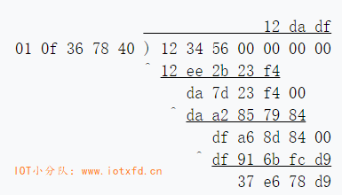
注意:多项式长除法概念的应用,但有几个重要的区别:在计算从除数中减去的伽罗华域的结果项/系数时,执行逐位无进位乘法,并使用所选的本原多项式与从第一次遇到的 MSB 进行异或获得“位流”结果,直到答案小于伽罗华域的值为止,在这种情况下为256。然后像往常一样执行 XOR “减法”。
以下演示这个操作方法(0x12 * 0x36):
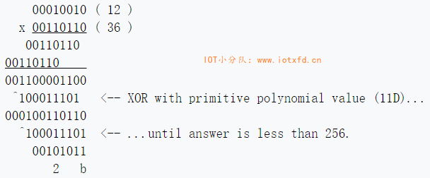
余数与信息连接,因此编码信息为12 34 56 37 e6 78 d9。
然而,长除法非常慢,因为它需要大量递归迭代才能终止。可以设计出更有效的策略,例如使用合成除法(也称为 Horner 的方法,可以在Khan Academy上找到一个很好的教程视频)。下面是实现$GF(2^p)$多项式的扩展合成除法的函数(扩展是因为除数是多项式而不是单项):
def gf_poly_div(dividend, divisor):
    '''Fast polynomial division by using Extended Synthetic Division and optimized for GF(2^p) computations
    (doesn't work with standard polynomials outside of this galois field, see the Wikipedia article for generic algorithm).'''
    # CAUTION: this function expects polynomials to follow the opposite convention at decoding:
    # the terms must go from the biggest to lowest degree (while most other functions here expect
    # a list from lowest to biggest degree). eg: 1 + 2x + 5x^2 = [5, 2, 1], NOT [1, 2, 5]

    msg_out = list(dividend) # Copy the dividend
    #normalizer = divisor[0] # precomputing for performance
    for i in range(0, len(dividend) - (len(divisor)-1)):
        #msg_out[i] /= normalizer # for general polynomial division (when polynomials are non-monic), the usual way of using
                                  # synthetic division is to divide the divisor g(x) with its leading coefficient, but not needed here.
        coef = msg_out[i] # precaching
        if coef != 0: # log(0) is undefined, so we need to avoid that case explicitly (and it's also a good optimization).
            for j in range(1, len(divisor)): # in synthetic division, we always skip the first coefficient of the divisior,
                                              # because it's only used to normalize the dividend coefficient
                if divisor[j] != 0: # log(0) is undefined
                    msg_out[i + j] ^= gf_mul(divisor[j], coef) # equivalent to the more mathematically correct
                                                               # (but xoring directly is faster): msg_out[i + j] += -divisor[j] * coef

    # The resulting msg_out contains both the quotient and the remainder, the remainder being the size of the divisor
    # (the remainder has necessarily the same degree as the divisor -- not length but degree == length-1 -- since it's
    # what we couldn't divide from the dividend), so we compute the index where this separation is, and return the quotient and remainder.
    separator = -(len(divisor)-1)
    return msg_out[:separator], msg_out[separator:] # return quotient, remainder.
下面是如何对消息进行编码以获得其 RS 码:
def rs_encode_msg(msg_in, nsym):
    '''Reed-Solomon main encoding function'''
    gen = rs_generator_poly(nsym)

    # Pad the message, then divide it by the irreducible generator polynomial
    _, remainder = gf_poly_div(msg_in + [0] * (len(gen)-1), gen)
    # The remainder is our RS code! Just append it to our original message to get our full codeword (this represents a polynomial of max 256 terms)
    msg_out = msg_in + remainder
    # Return the codeword
    return msg_out
很简单,不是吗?编码实际上是 Reed–Solomon 最简单的部分,它总是采用同样的方法(多项式除法)。解码是 Reed–Solomon 的艰难部分,根据你的需要,你会发现很多不同的算法,但我们稍后会讨论这个问题。
这个函数非常快,但是由于编码是非常关键的,下面是一个增强的编码函数,它包含多项式合成除法,这是 Reed–Solomon 软件库中最常见的形式:
def rs_encode_msg(msg_in, nsym):
    '''Reed-Solomon main encoding function, using polynomial division (algorithm Extended Synthetic Division)'''
    if (len(msg_in) + nsym) > 255: raise ValueError("Message is too long (%i when max is 255)" % (len(msg_in)+nsym))
    gen = rs_generator_poly(nsym)
    # Init msg_out with the values inside msg_in and pad with len(gen)-1 bytes (which is the number of ecc symbols).
    msg_out = [0] * (len(msg_in) + len(gen)-1)
    # Initializing the Synthetic Division with the dividend (= input message polynomial)
    msg_out[:len(msg_in)] = msg_in

    # Synthetic division main loop
    for i in range(len(msg_in)):
        # Note that it's msg_out here, not msg_in. Thus, we reuse the updated value at each iteration
        # (this is how Synthetic Division works: instead of storing in a temporary register the intermediate values,
        # we directly commit them to the output).
        coef = msg_out[i]

        # log(0) is undefined, so we need to manually check for this case. There's no need to check
        # the divisor here because we know it can't be 0 since we generated it.
        if coef != 0:
            # in synthetic division, we always skip the first coefficient of the divisior, because it's only used to normalize the dividend coefficient (which is here useless since the divisor, the generator polynomial, is always monic)
            for j in range(1, len(gen)):
                msg_out[i+j] ^= gf_mul(gen[j], coef) # equivalent to msg_out[i+j] += gf_mul(gen[j], coef)

    # At this point, the Extended Synthetic Divison is done, msg_out contains the quotient in msg_out[:len(msg_in)]
    # and the remainder in msg_out[len(msg_in):]. Here for RS encoding, we don't need the quotient but only the remainder
    # (which represents the RS code), so we can just overwrite the quotient with the input message, so that we get
    # our complete codeword composed of the message + code.
    msg_out[:len(msg_in)] = msg_in

    return msg_out
这个算法速度更快,但对于实际使用来说仍然很慢,特别是在 Python 中。有一些方法可以通过使用各种技巧来优化速度,例如内联(而不是gf_mul,代之以避免调用操作)、预计算(gen和coef的对数,甚至生成乘法表-但似乎后者在 Python 中不能很好地工作)、使用静态类型的构造(将gf_log和gf_exp分配给array.array('i', [...]))、使用内存视图(比如将所有列表更改为字节数组)、使用 PyPy 运行,或者将算法转换为 Cython 或 C 扩展。
此示例演示了应用于前面介绍的示例 QR 代码中的信息的编码函数。计算的纠错符号(在第二行上)匹配从 QR 码解码的值。
>>> msg_in = [ 0x40, 0xd2, 0x75, 0x47, 0x76, 0x17, 0x32, 0x06,
...            0x27, 0x26, 0x96, 0xc6, 0xc6, 0x96, 0x70, 0xec ]
>>> msg = rs_encode_msg(msg_in, 10)
>>> for i in range(0,len(msg)):
...    print(hex(msg[i]), end=' ')
...
0x40 0xd2 0x75 0x47 0x76 0x17 0x32 0x6 0x27 0x26 0x96 0xc6 0xc6 0x96 0x70 0xec
0xbc 0x2a 0x90 0x13 0x6b 0xaf 0xef 0xfd 0x4b 0xe0
Python 版本注意事项:
print hex(msg[i]),(包括最后逗号)并将range替换为xrange。
Reed–Solomon 解码是指从潜在损坏的消息和 RS 代码中返回经过修正的消息的过程。换句话说,解码是使用先前计算的 RS 码修复消息的过程。
虽然只有一种方法可以用 Reed–Solomon 对消息进行编码,但是有很多不同的解码方法,因此有很多不同的解码算法。
通常可以用 5 个步骤来描述解码过程。
下面我们将描述这五个步骤中的每一个步骤。
此外,解码器还可以按照它们可以修复的错误类型进行分类:擦除(知道损坏字符的位置,但不知道大小)、错误(忽略了位置和大小),或者这两种错误和擦除。我们将描述如何支持所有这些。
解码 Reed–Solomon 信息涉及几个步骤。第一步是计算信息的“综合征”。将该消息视为多项式,并在 $\alpha^0, \alpha^1, \alpha^2, ..., \alpha^n$ 处对其进行计算。由于这些都是生成多项式的零点,如果扫描的消息未损坏,则结果应为零(这可用于检查消息是否已损坏,以及在纠正已损坏的消息后是否已完全修复)。如果不是,综合征包含所有必要的信息,以确定应作出的纠正。编写一个计算综合征的函数是简单的。
def rs_calc_syndromes(msg, nsym):
    '''Given the received codeword msg and the number of error correcting symbols (nsym), computes the syndromes polynomial.
    Mathematically, it's essentially equivalent to a Fourrier Transform (Chien search being the inverse).
    '''
    # Note the "[0] +" : we add a 0 coefficient for the lowest degree (the constant). This effectively shifts the syndrome, and will shift every computations depending on the syndromes (such as the errors locator polynomial, errors evaluator polynomial, etc. but not the errors positions).
    # This is not necessary, you can adapt subsequent computations to start from 0 instead of skipping the first iteration (ie, the often seen range(1, n-k+1)),
    synd = [0] * nsym
    for i in range(0, nsym):
        synd[i] = gf_poly_eval(msg, gf_pow(2,i))
    return [0] + synd # pad with one 0 for mathematical precision (else we can end up with weird calculations sometimes)
继续这个例子,我们看到原始码元的综合征实际上是零。在消息或其 RS 码中引入至少一个字符的损坏会产生非零综合征。
>>> synd = rs_calc_syndromes(msg, 10)
>>> print(synd)
[0, 0, 0, 0, 0, 0, 0, 0, 0, 0] # not corrupted message = all 0 syndromes
>>> msg[0] = 0  # deliberately damage the message
>>> synd = rs_calc_syndromes(msg, 10)
>>> print(synd)
[64, 192, 93, 231, 52, 92, 228, 49, 83, 245] # when corrupted, the syndromes will be non zero
下面是自动检查的代码:
def rs_check(msg, nsym):
    '''Returns true if the message + ecc has no error of false otherwise (may not always catch a wrong decoding or a wrong message, particularly if there are too many errors -- above the Singleton bound --, but it usually does)'''
    return ( max(rs_calc_syndromes(msg, nsym)) == 0
如果错误的位置已经知道,那么纠正代码中的错误是最简单的。这就是所谓的擦除校正。对于添加到代码中的每个纠错符号,有可能校正一个被擦除的符号(如字符)。如果错误位置未知,则每个符号错误需要两个 EC 符号(这样您可以更正两次比擦除更小的错误)。这使得擦除校正在实践中很有用,如果正在扫描的部分 QR 码被覆盖或物理上被撕开。然而,扫码器可能很难确定是否发生了这种情况,因此并非所有的 QR 码扫码器都能执行擦除校正。
现在我们已经有了综合征,需要计算定位多项式。这很容易:
def rs_find_errata_locator(e_pos):
    '''Compute the erasures/errors/errata locator polynomial from the erasures/errors/errata positions
       (the positions must be relative to the x coefficient, eg: "hello worldxxxxxxxxx" is tampered to "h_ll_ worldxxxxxxxxx"
       with xxxxxxxxx being the ecc of length n-k=9, here the string positions are [1, 4], but the coefficients are reversed
       since the ecc characters are placed as the first coefficients of the polynomial, thus the coefficients of the
       erased characters are n-1 - [1, 4] = [18, 15] = erasures_loc to be specified as an argument.'''

    e_loc = [1] # just to init because we will multiply, so it must be 1 so that the multiplication starts correctly without nulling any term
    # erasures_loc = product(1 - x*alpha**i) for i in erasures_pos and where alpha is the alpha chosen to evaluate polynomials.
    for i in e_pos:
        e_loc = gf_poly_mul( e_loc, gf_poly_add([1], [gf_pow(2, i), 0]) )
    return e_loc
接下来,从定位多项式中计算擦除/错误评估多项式很容易,它只是一个多项式乘法和一个多项式除法(您可以用列表切片代替它,因为这是我们最后想要的效果):
def rs_find_error_evaluator(synd, err_loc, nsym):
    '''Compute the error (or erasures if you supply sigma=erasures locator polynomial, or errata) evaluator polynomial Omega
       from the syndrome and the error/erasures/errata locator Sigma.'''

    # Omega(x) = [ Synd(x) * Error_loc(x) ] mod x^(n-k+1)
    _, remainder = gf_poly_div( gf_poly_mul(synd, err_loc), ([1] + [0]*(nsym+1)) ) # first multiply syndromes * errata_locator, then do a  polynomial division to truncate the polynomial to the required length

    # Faster way that is equivalent
    # remainder = gf_poly_mul(synd, err_loc) # first multiply the syndromes with the errata locator polynomial
    # remainder = remainder[len(remainder)-(nsym+1):] # then slice the list to truncate it (which represents the polynomial), which is equivalent to dividing by a polynomial of the length we want

    return remainder
最后,利用 Forney 算法计算校正值(也称为误差幅度多项式)。它是在下面的函数中实现的。
def rs_correct_errata(msg_in, synd, err_pos): # err_pos is a list of the positions of the errors/erasures/errata
    '''Forney algorithm, computes the values (error magnitude) to correct the input message.'''
    # calculate errata locator polynomial to correct both errors and erasures (by combining the errors positions given by the error locator polynomial found by BM with the erasures positions given by caller)
    coef_pos = [len(msg_in) - 1 - p for p in err_pos] # need to convert the positions to coefficients degrees for the errata locator algo to work (eg: instead of [0, 1, 2] it will become [len(msg)-1, len(msg)-2, len(msg) -3])
    err_loc = rs_find_errata_locator(coef_pos)
    # calculate errata evaluator polynomial (often called Omega or Gamma in academic papers)
    err_eval = rs_find_error_evaluator(synd[::-1], err_loc, len(err_loc)-1)[::-1]

    # Second part of Chien search to get the error location polynomial X from the error positions in err_pos (the roots of the error locator polynomial, ie, where it evaluates to 0)
    X = [] # will store the position of the errors
    for i in range(0, len(coef_pos)):
        l = 255 - coef_pos[i]
        X.append( gf_pow(2, -l) )

    # Forney algorithm: compute the magnitudes
    E = [0] * (len(msg_in)) # will store the values that need to be corrected (substracted) to the message containing errors. This is sometimes called the error magnitude polynomial.
    Xlength = len(X)
    for i, Xi in enumerate(X):

        Xi_inv = gf_inverse(Xi)

        # Compute the formal derivative of the error locator polynomial (see Blahut, Algebraic codes for data transmission, pp 196-197).
        # the formal derivative of the errata locator is used as the denominator of the Forney Algorithm, which simply says that the ith error value is given by error_evaluator(gf_inverse(Xi)) / error_locator_derivative(gf_inverse(Xi)). See Blahut, Algebraic codes for data transmission, pp 196-197.
        err_loc_prime_tmp = []
        for j in range(0, Xlength):
            if j != i:
                err_loc_prime_tmp.append( gf_sub(1, gf_mul(Xi_inv, X[j])) )
        # compute the product, which is the denominator of the Forney algorithm (errata locator derivative)
        err_loc_prime = 1
        for coef in err_loc_prime_tmp:
            err_loc_prime = gf_mul(err_loc_prime, coef)
        # equivalent to: err_loc_prime = functools.reduce(gf_mul, err_loc_prime_tmp, 1)

        # Compute y (evaluation of the errata evaluator polynomial)
        # This is a more faithful translation of the theoretical equation contrary to the old forney method. Here it is an exact reproduction:
        # Yl = omega(Xl.inverse()) / prod(1 - Xj*Xl.inverse()) for j in len(X)
        y = gf_poly_eval(err_eval[::-1], Xi_inv) # numerator of the Forney algorithm (errata evaluator evaluated)
        y = gf_mul(gf_pow(Xi, 1), y)

        # Check: err_loc_prime (the divisor) should not be zero.
        if err_loc_prime == 0:
            raise ReedSolomonError("Could not find error magnitude")    # Could not find error magnitude

        # Compute the magnitude
        magnitude = gf_div(y, err_loc_prime) # magnitude value of the error, calculated by the Forney algorithm (an equation in fact): dividing the errata evaluator with the errata locator derivative gives us the errata magnitude (ie, value to repair) the ith symbol
        E[err_pos[i]] = magnitude # store the magnitude for this error into the magnitude polynomial

    # Apply the correction of values to get our message corrected! (note that the ecc bytes also gets corrected!)
    # (this isn't the Forney algorithm, we just apply the result of decoding here)
    msg_in = gf_poly_add(msg_in, E) # equivalent to Ci = Ri - Ei where Ci is the correct message, Ri the received (senseword) message, and Ei the errata magnitudes (minus is replaced by XOR since it's equivalent in GF(2^p)). So in fact here we substract from the received message the errors magnitude, which logically corrects the value to what it should be.
    return msg_in
数学注解:误差值表达式的分母是错误定位多项式 q 的形式导数,这通常是用$n c_n x^{n-1}$代替每个项$c_n x^n$的过程来计算的。由于我们工作在一个第二特征域,当 n 是奇数时,$nc_n$等于$c_n$,当 n 是偶数时,n 的值为 0。因此,我们可以简单地去除偶数系数(导致多项式
qprime)并计算 $qprime(x^2)$。
Python 注解:该函数使用
[::-1]反转列表中元素的顺序。这是必要的,因为函数并不都使用相同的排序约定(例如,有些先使用最少的项,另一些先使用最大的项)。它还使用了列表推导式,这只是编写for循环的一种简洁方法,其中的条目被附加到列表中,但是 Python 解释器可以对其进行比循环更多的优化。
继续这个例子,这里我们使用rs_correct_errata来恢复消息的第一个字节。
>>> msg[0] = 0
>>> synd = rs_calc_syndromes(msg, 10)
>>> msg = rs_correct_errata(msg, synd, [0]) # [0] is the list of the erasures locations, here it's the first character, at position 0
>>> print(hex(msg[0]))
0x40
在更可能的情况下,错误位置未知(通常称之为错误,而不是已知位置的擦除),我们将使用与擦除相同的步骤,但现在需要额外的步骤来查找位置。Berlekamp–Massey 算法用于计算错误定位多项式,稍后我们可以使用它来确定错误位置:
def rs_find_error_locator(synd, nsym, erase_loc=None, erase_count=0):
    '''Find error/errata locator and evaluator polynomials with Berlekamp-Massey algorithm'''
    # The idea is that BM will iteratively estimate the error locator polynomial.
    # To do this, it will compute a Discrepancy term called Delta, which will tell us if the error locator polynomial needs an update or not
    # (hence why it's called discrepancy: it tells us when we are getting off board from the correct value).

    # Init the polynomials
    if erase_loc: # if the erasure locator polynomial is supplied, we init with its value, so that we include erasures in the final locator polynomial
        err_loc = list(erase_loc)
        old_loc = list(erase_loc)
    else:
        err_loc = [1] # This is the main variable we want to fill, also called Sigma in other notations or more formally the errors/errata locator polynomial.
        old_loc = [1] # BM is an iterative algorithm, and we need the errata locator polynomial of the previous iteration in order to update other necessary variables.
    #L = 0 # update flag variable, not needed here because we use an alternative equivalent way of checking if update is needed (but using the flag could potentially be faster depending on if using length(list) is taking linear time in your language, here in Python it's constant so it's as fast.

    # Fix the syndrome shifting: when computing the syndrome, some implementations may prepend a 0 coefficient for the lowest degree term (the constant). This is a case of syndrome shifting, thus the syndrome will be bigger than the number of ecc symbols (I don't know what purpose serves this shifting). If that's the case, then we need to account for the syndrome shifting when we use the syndrome such as inside BM, by skipping those prepended coefficients.
    # Another way to detect the shifting is to detect the 0 coefficients: by definition, a syndrome does not contain any 0 coefficient (except if there are no errors/erasures, in this case they are all 0). This however doesn't work with the modified Forney syndrome, which set to 0 the coefficients corresponding to erasures, leaving only the coefficients corresponding to errors.
    synd_shift = 0
    if len(synd) > nsym: synd_shift = len(synd) - nsym

    for i in range(0, nsym-erase_count): # generally: nsym-erase_count == len(synd), except when you input a partial erase_loc and using the full syndrome instead of the Forney syndrome, in which case nsym-erase_count is more correct (len(synd) will fail badly with IndexError).
        if erase_loc: # if an erasures locator polynomial was provided to init the errors locator polynomial, then we must skip the FIRST erase_count iterations (not the last iterations, this is very important!)
            K = erase_count+i+synd_shift
        else: # if erasures locator is not provided, then either there's no erasures to account or we use the Forney syndromes, so we don't need to use erase_count nor erase_loc (the erasures have been trimmed out of the Forney syndromes).
            K = i+synd_shift

        # Compute the discrepancy Delta
        # Here is the close-to-the-books operation to compute the discrepancy Delta: it's a simple polynomial multiplication of error locator with the syndromes, and then we get the Kth element.
        #delta = gf_poly_mul(err_loc[::-1], synd)[K] # theoretically it should be gf_poly_add(synd[::-1], [1])[::-1] instead of just synd, but it seems it's not absolutely necessary to correctly decode.
        # But this can be optimized: since we only need the Kth element, we don't need to compute the polynomial multiplication for any other element but the Kth. Thus to optimize, we compute the polymul only at the item we need, skipping the rest (avoiding a nested loop, thus we are linear time instead of quadratic).
        # This optimization is actually described in several figures of the book "Algebraic codes for data transmission", Blahut, Richard E., 2003, Cambridge university press.
        delta = synd[K]
        for j in range(1, len(err_loc)):
            delta ^= gf_mul(err_loc[-(j+1)], synd[K - j]) # delta is also called discrepancy. Here we do a partial polynomial multiplication (ie, we compute the polynomial multiplication only for the term of degree K). Should be equivalent to brownanrs.polynomial.mul_at().
        #print "delta", K, delta, list(gf_poly_mul(err_loc[::-1], synd)) # debugline

        # Shift polynomials to compute the next degree
        old_loc = old_loc + [0]

        # Iteratively estimate the errata locator and evaluator polynomials
        if delta != 0: # Update only if there's a discrepancy
            if len(old_loc) > len(err_loc): # Rule B (rule A is implicitly defined because rule A just says that we skip any modification for this iteration)
            #if 2*L <= K+erase_count: # equivalent to len(old_loc) > len(err_loc), as long as L is correctly computed
                # Computing errata locator polynomial Sigma
                new_loc = gf_poly_scale(old_loc, delta)
                old_loc = gf_poly_scale(err_loc, gf_inverse(delta)) # effectively we are doing err_loc * 1/delta = err_loc // delta
                err_loc = new_loc
                # Update the update flag
                #L = K - L # the update flag L is tricky: in Blahut's schema, it's mandatory to use `L = K - L - erase_count` (and indeed in a previous draft of this function, if you forgot to do `- erase_count` it would lead to correcting only 2*(errors+erasures) <= (n-k) instead of 2*errors+erasures <= (n-k)), but in this latest draft, this will lead to a wrong decoding in some cases where it should correctly decode! Thus you should try with and without `- erase_count` to update L on your own implementation and see which one works OK without producing wrong decoding failures.

            # Update with the discrepancy
            err_loc = gf_poly_add(err_loc, gf_poly_scale(old_loc, delta))

    # Check if the result is correct, that there's not too many errors to correct
    while len(err_loc) and err_loc[0] == 0: del err_loc[0] # drop leading 0s, else errs will not be of the correct size
    errs = len(err_loc) - 1
    if (errs-erase_count) * 2 + erase_count > nsym:
        raise ReedSolomonError("Too many errors to correct")    # too many errors to correct

    return err_loc
然后,使用错误定位多项式,我们简单地使用一种称为试换法的暴力方法来查找该多项式的零,该方法识别错误位置(即需要更正的字符的索引)。存在一种更有效的算法,称为 Chien 搜索,它避免了在每次迭代时重新计算整个评估,但该算法作为练习留给读者。
def rs_find_errors(err_loc, nmess): # nmess is len(msg_in)
    '''Find the roots (ie, where evaluation = zero) of error polynomial by brute-force trial, this is a sort of Chien's search
    (but less efficient, Chien's search is a way to evaluate the polynomial such that each evaluation only takes constant time).'''
    errs = len(err_loc) - 1
    err_pos = []
    for i in range(nmess): # normally we should try all 2^8 possible values, but here we optimize to just check the interesting symbols
        if gf_poly_eval(err_loc, gf_pow(2, i)) == 0: # It's a 0? Bingo, it's a root of the error locator polynomial,
                                                                                   # in other terms this is the location of an error
            err_pos.append(nmess - 1 - i)
    # Sanity check: the number of errors/errata positions found should be exactly the same as the length of the errata locator polynomial
    if len(err_pos) != errs:
        # couldn't find error locations
        raise ReedSolomonError("Too many (or few) errors found by Chien Search for the errata locator polynomial!")
    return err_pos
数学注解:当错误定位多项式是线性的(
err_poly长度为 2)时,它可以很容易地求解,而不需要借助蛮力方法。上述功能没有利用这一事实,但感兴趣的读者可能希望实现更有效的解决方案。同样,当错误定位器是二次元时,可以用二次公式的推广来求解。更有雄心的读者也可能希望实施这一程序。
下面是一个示例,其中更正了消息中的三个错误:
>>> print(hex(msg[10]))
0x96
>>> msg[0] = 6
>>> msg[10] = 7
>>> msg[20] = 8
>>> synd = rs_calc_syndromes(msg, 10)
>>> err_loc = rs_find_error_locator(synd, nsym)
>>> pos = rs_find_errors(err_loc[::-1], len(msg)) # find the errors locations
>>> print(pos)
[20, 10, 0]
>>> msg = rs_correct_errata(msg, synd, pos)
>>> print(hex(msg[10]))
0x96
Reed–Solomon 译码器可以同时对擦除和错误进行解码,最大限度(称为 Singleton Bound)为 $2*e+v <= (n-k)$,其中$e$是错误数,$v$是擦除数,$(n-k)$是 RS 码字符数(代码中为nsym)。基本上,这意味着对于每一个擦除,您只需要一个 RS 码字符来修复它,而对于每一个错误,您需要两个 RS 码字符(因为您需要找到除了值/大小之外的位置来更正)。这种解码器被称为错误与擦除解码器,或勘误解码器。
为了纠正错误和擦除,我们必须防止擦除干扰错误定位过程。这可以通过计算 Forney 综合征来实现,如下所示。
def rs_forney_syndromes(synd, pos, nmess):
    # Compute Forney syndromes, which computes a modified syndromes to compute only errors (erasures are trimmed out). Do not confuse this with Forney algorithm, which allows to correct the message based on the location of errors.
    erase_pos_reversed = [nmess-1-p for p in pos] # prepare the coefficient degree positions (instead of the erasures positions)

    # Optimized method, all operations are inlined
    fsynd = list(synd[1:])      # make a copy and trim the first coefficient which is always 0 by definition
    for i in range(0, len(pos)):
        x = gf_pow(2, erase_pos_reversed[i])
        for j in range(0, len(fsynd) - 1):
            fsynd[j] = gf_mul(fsynd[j], x) ^ fsynd[j + 1]

    # Equivalent, theoretical way of computing the modified Forney syndromes: fsynd = (erase_loc * synd) % x^(n-k)
    # See Shao, H. M., Truong, T. K., Deutsch, L. J., & Reed, I. S. (1986, April). A single chip VLSI Reed-Solomon decoder. In Acoustics, Speech, and Signal Processing, IEEE International Conference on ICASSP'86. (Vol. 11, pp. 2151-2154). IEEE.ISO 690
    #erase_loc = rs_find_errata_locator(erase_pos_reversed, generator=generator) # computing the erasures locator polynomial
    #fsynd = gf_poly_mul(erase_loc[::-1], synd[1:]) # then multiply with the syndrome to get the untrimmed forney syndrome
    #fsynd = fsynd[len(pos):] # then trim the first erase_pos coefficients which are useless. Seems to be not necessary, but this reduces the computation time later in BM (thus it's an optimization).

    return fsynd
然后,在错误定位过程中,可以使用 Forney 综合征代替常规综合征。
下面的函数rs_correct_msg将完整的过程组合在一起。擦除是通过提供擦除erase_pos来指示的,这是信息msg_in(完整接收的信息:原始消息 + ecc)中的擦除索引位置的列表。
def rs_correct_msg(msg_in, nsym, erase_pos=None):
    '''Reed-Solomon main decoding function'''
    if len(msg_in) > 255: # can't decode, message is too big
        raise ValueError("Message is too long (%i when max is 255)" % len(msg_in))

    msg_out = list(msg_in)     # copy of message
    # erasures: set them to null bytes for easier decoding (but this is not necessary, they will be corrected anyway, but debugging will be easier with null bytes because the error locator polynomial values will only depend on the errors locations, not their values)
    if erase_pos is None:
        erase_pos = []
    else:
        for e_pos in erase_pos:
            msg_out[e_pos] = 0
    # check if there are too many erasures to correct (beyond the Singleton bound)
    if len(erase_pos) > nsym: raise ReedSolomonError("Too many erasures to correct")
    # prepare the syndrome polynomial using only errors (ie: errors = characters that were either replaced by null byte
    # or changed to another character, but we don't know their positions)
    synd = rs_calc_syndromes(msg_out, nsym)
    # check if there's any error/erasure in the input codeword. If not (all syndromes coefficients are 0), then just return the message as-is.
    if max(synd) == 0:
        return msg_out[:-nsym], msg_out[-nsym:]  # no errors

    # compute the Forney syndromes, which hide the erasures from the original syndrome (so that BM will just have to deal with errors, not erasures)
    fsynd = rs_forney_syndromes(synd, erase_pos, len(msg_out))
    # compute the error locator polynomial using Berlekamp-Massey
    err_loc = rs_find_error_locator(fsynd, nsym, erase_count=len(erase_pos))
    # locate the message errors using Chien search (or brute-force search)
    err_pos = rs_find_errors(err_loc[::-1] , len(msg_out))
    if err_pos is None:
        raise ReedSolomonError("Could not locate error")    # error location failed

    # Find errors values and apply them to correct the message
    # compute errata evaluator and errata magnitude polynomials, then correct errors and erasures
    msg_out = rs_correct_errata(msg_out, synd, (erase_pos + err_pos)) # note that we here use the original syndrome, not the forney syndrome
                                                                                                                                  # (because we will correct both errors and erasures, so we need the full syndrome)
    # check if the final message is fully repaired
    synd = rs_calc_syndromes(msg_out, nsym)
    if max(synd) > 0:
        raise ReedSolomonError("Could not correct message")     # message could not be repaired
    # return the successfully decoded message
    return msg_out[:-nsym], msg_out[-nsym:] # also return the corrected ecc block so that the user can check()
Python 注解:列表
erase_pos与err_pos使用+号连接。
这是一个完整操作的纠错和擦除 Reed–Solomon 解码器所需要的最后一块。如果你想深入研究勘误(错误和擦除)解码器的内部工作,你可以阅读 Richard E. Blahut 的优秀著作“数据传输的代数码”(2003)。
数学注解:在一些软件实现中,特别是使用为线性代数和矩阵操作优化的语言的软件实现中,您会发现算法(编码、Berlekamp-Massey 等)会看起来完全不同并使用傅里叶变换。因为这是完全等价的:用频谱估计的行话说,解码 Reed–Solomn 由一个傅里叶变换(综合征计算机),然后是频谱分(Berlekamp-Massey 或欧几里得算法),然后是逆傅里叶变换(Chien 搜索)。事实上,如果您使用的是为线性代数优化的编程语言,或者如果您想使用快速线性代数库,那么使用傅里叶变换是一个非常好的主意,因为它现在非常快(特别是快速傅里叶变换或数论变换[5])。
下面是一个示例,说明如何使用您刚刚完成的函数,以及如何对错误和擦除进行解码。
# Configuration of the parameters and input message
prim = 0x11d
n = 20 # set the size you want, it must be > k, the remaining n-k symbols will be the ECC code (more is better)
k = 11 # k = len(message)
message = "hello world" # input message

# Initializing the log/antilog tables
init_tables(prim)

# Encoding the input message
mesecc = rs_encode_msg([ord(x) for x in message], n-k)
print("Original: %s" % mesecc)

# Tampering 6 characters of the message (over 9 ecc symbols, so we are above the Singleton Bound)
mesecc[0] = 0
mesecc[1] = 2
mesecc[2] = 2
mesecc[3] = 2
mesecc[4] = 2
mesecc[5] = 2
print("Corrupted: %s" % mesecc)

# Decoding/repairing the corrupted message, by providing the locations of a few erasures, we get below the Singleton Bound
# Remember that the Singleton Bound is: 2*e+v <= (n-k)
corrected_message, corrected_ecc = rs_correct_msg(mesecc, n-k, erase_pos=[0, 1, 2])
print("Repaired: %s" % (corrected_message+corrected_ecc))
print(''.join([chr(x) for x in corrected_message]))
输出如下:
Original:  [104, 101, 108, 108, 111,  32, 119, 111, 114, 108, 100, 145, 124, 96, 105, 94, 31, 179, 149, 163]
Corrupted: [  0,   2,   2,   2,   2,   2, 119, 111, 114, 108, 100, 145, 124, 96, 105, 94, 31, 179, 149, 163]
Repaired:  [104, 101, 108, 108, 111,  32, 119, 111, 114, 108, 100, 145, 124, 96, 105, 94, 31, 179, 149, 163]
hello world
本文介绍了 Reed–Solomon 码的基本原理。已经包含了用于特定实现的 Python 代码(使用通用 Reed–Solomon 编解码器来纠正误读的 QR 码)。这里介绍的代码是相当通用的,可以用于 QR 码之外的任何用途,在 QR 码中,您需要更正错误/擦除,例如文件保护、网络等,这些思想的许多变化和改进是可能的,因为编码理论是一个非常丰富的研究领域。
如果您的代码只是针对自己的数据(例如,您希望能够生成和读取您自己的 QR 码),那没有问题。如果您使用他人提供的数据(例如,您希望读取和解码其他应用程序的 QR 码),那么这个解码器可能是不够的,因为这里有一些隐藏的参数是为了简单而固定的(即:生成器/alpha 数和第一个连续的根)。如果你想解码由其他库生成的 Reed–Solomon 代码,将需要使用通用的 Reed–Solomon 编解码器,这将允许指定你自己的参数,甚至超越域$2^8$。
在补充资源页面上,您将找到一个扩展的通用版本的代码,可以使用它来解码几乎所有的 Reed–Solomon 代码,同时还可以生成主多项式列表,以及检测未知 RS 代码参数的算法。请注意,无论您使用什么参数,修复功能都应该是相同的:为 log/antilog 表和生成多项式生成的值不会更改 Reed–Solomon 码的结构,因此无论参数是什么,您总是得到相同的功能。
您可能已经注意到的一个直接问题是,我们只能编码 256 个字符的消息。这个限制可以通过几种方法来规避,其中最常见的有三种:
如果你想更进一步的话,有很多关于 Reed–Solomon 码的书籍和科学文章,一个很好的起点是作者 Richard Blahut,他在这一领域很有名。此外, Reed–Solomon 码有很多不同的编码和解码方式,因此你会发现很多不同的算法,尤其是用于解码的算法(Berlekamp-Massey, Berlekamp-Welch, 欧几里得算法等等)。
如果您希望更高的的性能,将在文献中发现几个变体的算法,如 Cauchy–Reed–Solomon。编程实现对 Reed–Solomon 编解码器的性能也起着很大的作用,这会导致 1000 倍的速度差异。欲了解更多信息,请阅读额外资源的“优化性能”。
即使当前最优秀的前向纠错算法现在都很流行(如LDPC码、Turbo码等)。因为他们速度快,Reed–Solomon 是最理想的FEC,这意味着它可以达到理论极限,即单例极限。实际上,这意味着 RS 可以同时更正最多$2*e+v <= (n-k)$错误和擦除,其中 e 是错误数,v 是擦除数,k 是消息大小,n 是消息+编码尺寸和$(n-k)$最小距离。这并不是说接近最佳的 FEC 是无用的:它们比 Reed–Solomon 可能的速度快得难以想象,而且它们可能更少地受到悬崖效应的影响(这意味着,即使有太多错误无法纠正所有错误,他们仍可能部分地解码消息的一部分,这与 RS 相反,RS 肯定会失败,甚至会悄悄地解码错误的消息而不被检测到)。但他们肯定无法纠正 Reed–Solomon 那样多的错误。在接近最优的 FEC 和最优的 FEC 之间进行选择主要是速度的问题。
最近,Reed–Solomon 的研究领域从 w:List_decoding(不与软解码混淆)的发现中恢复了一些活力,它允许对更多的符号进行解码/修复,超过了理论上的最佳限制。其核心思想是,只做解码,而不是标准 Reed–Solomon(这意味着它总是导致一个单一的解决方案,如果它不能,因为它超过理论限制,解码器将返回一个错误或错误的结果)。Reed–Solomon 的列表解码仍然会试图超越极限,并得到一些可能的结果,但通过巧妙地检查不同的结果,它往往可能只区分一个多项式,这可能是正确的。
一些列表解码算法已经可用,允许最多修复 $n-\sqrt{n\times k}$,而不是 $2\times e+v <= (n-k)$,其他列表解码算法(更高效或更多的符号解码)目前正在研究中。
;